FlashGPU-sim: Enabling GPU Modeling for Modern Architectures and AI Workloads
论文链接:《FlashGPU-sim: Enabling GPU Modeling for Modern Architectures and AI Workloads》
仓库链接:FlashGPU-Sim
BackGround: 当前 NVIDIA 厂家在内的 GPU 底层硬件架构处于黑盒状态,无论是做软件 kernel 的性能调优还是硬件层面的优化,均需要一个良好(high fidelity)的模拟器来定量测试。目前已知的 GPU 模拟器(包括 GPGPU 等)均是面向 Amphere 及其之前的 GPU 架构设计的,对于 Hopper 与 Blackwell 架构中新添加的许多重要的硬件 mechanism 不予支持,需要新的模拟器来补齐这一差距。
主要补充的 mechanism 包括:
- TMA( Tensor Memory Accelerator ) 异步数据搬运;
- Asynchronous Memory Barrier(用于 Data Movement 同步);
- DSMEM( Distributed Shared Memory ) 分布式共享内存;
- 在 SM 上方增加 GPC 这一组织层级(夹着 TPC 与 CPC 两个 layers);
- Tensor Core 演进,从
mma到 Hopper 架构wgmma到 Blackwell 架构tcgen05.
1.1 对 TMA 的建模
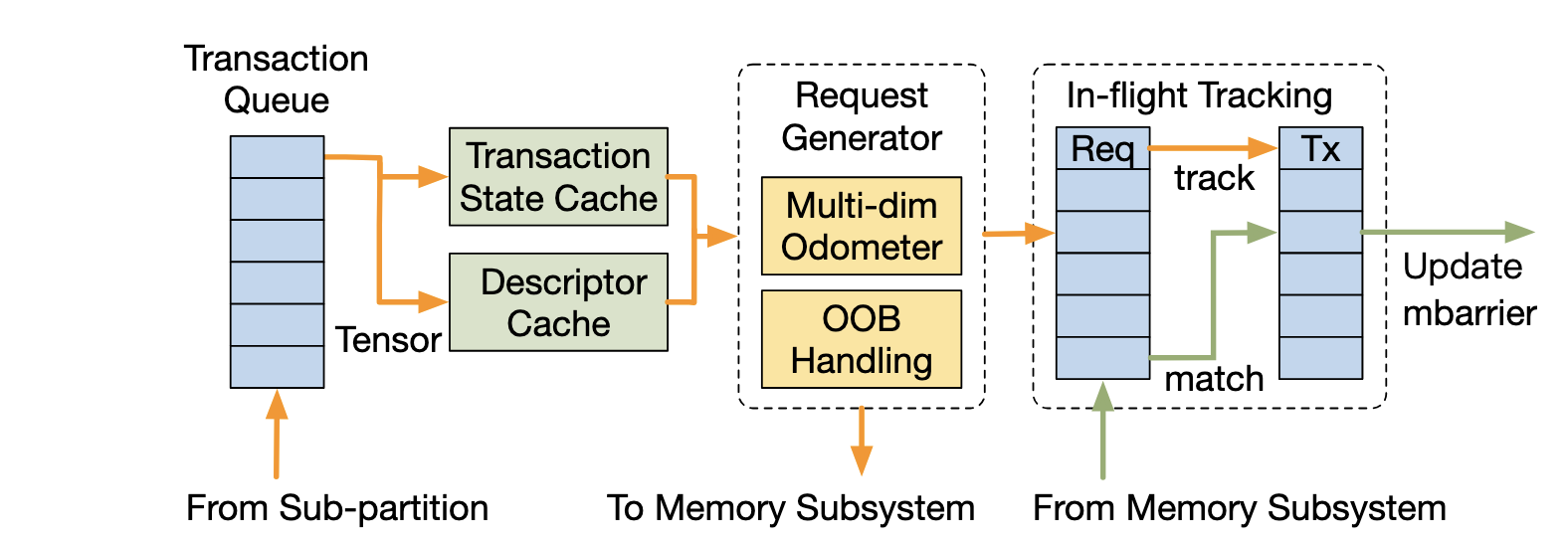
TMA 是单个 SM 独有,四个 sub-partion 共享。单个 cp.async.bulk 指令作为一个 TMA Transaction,传输的数据量是变长的,需要拆分为若干个等长的 request 一个一个 issue. 这里 descriptor cache 就是从 global memory 加载到 shared memory 的 cuTensorMap,提高重复访问的效率。注意,普通的 cp.async.bulk 不需要 cuTensorMap,只有 cp.async.bulk.tensor 才需要。
在做 benchmark 的时候可以学习一下:
- independent operation chain 可以测量单个 operation 的 issue gap;
- dependent operation chain 可以测量单个 operation 的 latency;
- 如果有 transaction cache 或者 issue slot 这样的有限结构,可以由单个 warp 连续 issue 或者多个 warp 同时 issue,测量 cache 或者 slot 的容量(最好要使单个 operation 时间稍微长一点,始终处于 in-flight 的状态)。
比如,对于 transaction cache 容量,benchmark 测试结果为:
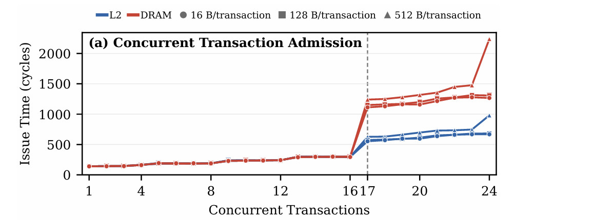
除了 transaction cache 容量,还测试:
- TMA pipeline throughput,平均每周期 issue 的 request 对应的字节数;
- 根据 in-flight requests 数量以及单个 request 延迟推断 In-flight Tracking 所能记录的 request 最大数量;
- 处理越界数据的方法:for write,不会产生 request;for read,request 最多到达 L2 Cache,不会到 DRAM.
文章中提到 Little's Law(利特尔法则)基本原理,一个稳定系统中:
其中:
- \(L\):系统中平均同时存在的任务数量;
- \(\lambda\):平均到达或完成速率;
- \(W\):每个任务在系统中停留的平均时间。
即:
并发数量 = 每周期处理多少请求 × 每个请求要停留多少周期。
1.2 Asynchronous Memory Barrier
主要测量 mbarrier 轮询的周期数,轮询主要包含两类 test_wait 与 try_wait:
| Wait Form | SASS Pattern | Latency( cycles ) |
|---|---|---|
| test wait | PHASECHK | 42 |
| try wait + nohint | PHASECHK.TRYWAIT | 42 |
| try wait + hint, complete | TRYWAIT + SLEEP + PHASECHK | 150 |
| try wait + hint, uncomplete | TRYWAIT + SLEEP + PHASECHK | hint dependent |
1.3 Evolving Tensor Core
从先前架构的 mma 到 Hopper 架构的 wgmma 到 Blackwell 架构的 tagen05,tensor core 的计算组织在不断变化,文章里提到如何从某一个架构的 SPEC 手册里面提取 tensor core 的理论算力信息。
Let \(T_{\mathrm{chip}}\) denote the peak dense tensor throughput in \(\mathrm{TOPS}\) and \(S\) the number of SMs. An mma.sync of shape \(M \times N \times K\) performs \(2M N K\) operations, giving the theoretical per-SM issue gap:
where \(f\) is the SM clock frequency in \(\mathrm{GHz}\). Since each SM contains \(P=4\) tensor-core sub-partitions, the corresponding single-warp theoretical gap is \(\mathrm{Gap}^{\mathrm{theo}}_{\mathrm{warp}} = P \times \mathrm{Gap}^{\mathrm{theo}}_{\mathrm{SM}}\).
实际的 Gap 和 Latency 通过 benchmark 测量。wgmma 和 tcgen05 有一个共同的 tensor core 算力模型,文章提到【For each operation, its workload of \(2M N K\) \(\mathrm{FLOPs}\) is converted into a compute service time using a data-type-specific per-SM service rate. Based on our measurements, the FP16 service rate is set to \(4096~\mathrm{FLOP/SM/cycle}\) on H100 and \(8192~\mathrm{FLOP/SM/cycle}\) on B200. All concurrent tensor operations on the same SM share this service capacity, bounding their aggregate compute throughput by the configured rate.】也就是单个 SM 的算力是各个 warp 共享的,尽管实际各个 warp 的 wgmma 或者 tcgen05 是并发的还是并行的未可知,但是基于该 capacity 的建模是较为准确的。
1.4 分布式共享内存
根据 NVIDIA DSMEM patent 构建的模型如图:
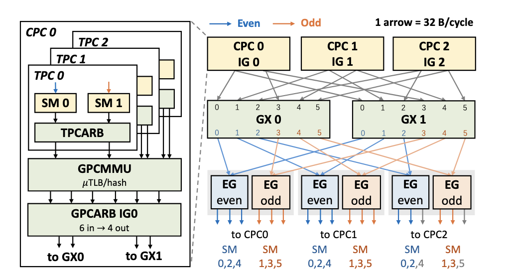
SM 的组织层次也比较清楚了,两个 SM 组成一个 TPC( Texture Processing Unit ),三个 TPC 组成一个 CPC( Compute Processing Unit ),三个 CPC 组成一个 GPC( Graphic Processing Unit ). 所以一个满配的 GPC 包含 \(18\) 个 SM.
DSM 性能不仅取决于链路带宽,还强烈取决于流量方向、发送源是否相同,以及反向回复流量的大小。可观测规律包含:
- 远端访问有明显固定开销:SM-to-SM 单向约 \(78~\mathrm{cycles}\),依赖型 remote load 往返约 \(220~\mathrm{cycles}\),remote store 可见约 \(625~\mathrm{cycles}\);
- 每个 SM 有独立的发送上限,约 \(21~\mathrm{B/cycle}\),不能借用空闲邻居 SM 的带宽;
- 同一 SM 发出的同方向流量共享 send budget,总吞吐基本不会超过约 \(21~\mathrm{B/cycle}\);
- 相反方向的流量由不同 SM 分别发送,可以利用两个 send budget,因此吞吐更高;
- Remote load 包含读请求和较大的反向数据回复,SM1 与 SM2 双向访问时 request/reply 竞争严重,每方向吞吐下降约 \(23\%\);
- Store 和 TMA put 的反向流量主要是可合并 ACK,因此 SM1 与 SM2 互相访问时双向竞争较轻,每方向仅下降约 \(4\% \sim 5\%\);
注意:上述依赖型 remote load 或者 remote store 的计算逻辑是 \(T_{\mathrm{remote}} = T_{\mathrm{local}}+T_{\mathrm{remote}}^{\mathrm{request}}+T_{\mathrm{remote}}^{\mathrm{reply}}\),其中 \(T_{\mathrm{local}}\) 是 SM 读写本地 shared memory 的固有开销,剩下两段 request 和 reply 是 remote 额外的 overhead. 而单个 \(T_{\mathrm{remote}}^{\mathrm{request}}\) 与 \(T_{\mathrm{remote}}^{\mathrm{reply}}\) 就是 SM-to-SM 的单向约 \(78~\mathrm{cycles}\) 的开销。
FlashGPU-Sim 因而采用“每个 SM 一个发送预算,request queue 和 reply queue 共同竞争”的模型,可以较好地模拟上述约束。
此外,FlashGPU-Sim 本身是 execution-driven, cycle-accurate 的模拟器。
当前主流的 GPU 模拟器分为 execution-driven 与 trace-driven:
- Execution-driven 在模拟过程中执行程序并动态产生指令流;
- Trace-driven 预先记录真实硬件的动态指令流,模拟时只重放。
比如执行一段 while( cond ){ } 循环,对于 execution-driven 的模拟器,其会按照编译好的 PTX 汇编指令逐条执行分支指令,实时判断是否应该跳转;对于 trace-driven 的模拟器,其会首先在一块 GPU 卡上运行一遍 kernel,记录好每一个 warp 执行的 SASS 指令流,然后再在模拟器里面按顺序重放。
Trace-driven 模拟器有两个缺陷。其一,如果指令流中出现异步指令,比如 mbarrier 的结束是隐式的,无法追踪到。其二,如果要做硬件参数的调整或者硬件部件的增减,已有的 GPU 计算卡做不了自然也就得不到 SASS 指令流,trace-driven 的模拟器也就无法重放,还是上面的例子,如果因为硬件参数的变化使得 while( ) 循环结束的时间改变,trace-driven 的模拟器感知不到。
当开启 GPC cluster 这一层级时,CPU 上绑核的单 thread 模拟一个 GPC 内的逻辑;未开启 GPC cluster 这一级时,CPU 上绑核的单 thread 模拟一个 SM 内的逻辑。对于 FlashGPU-Sim 的另一个特性:cycle-accurate. 处理的方式如下:
- 在 Simulated Cycle \(t\) 中
- 并行计算阶段
- \(\mathrm{SM}_0/\mathrm{GPC}_0\) 推进计算,产生通信/访存请求;
- \(\mathrm{SM}_1/\mathrm{GPC}_1\) 推进计算,产生通信/访存请求;
- \(\mathrm{SM}_2/\mathrm{GPC}_2\) 推进计算,产生通信/访存请求;
- \(\cdots\)
- 同步点
- 确定性共享资源阶段
- DSM fabric 每个 GPC 推进一个 cycle;
- Crossbar Arbitration 推进一个 cycle;
- Interconnect 推进一个 cycle;
- L2 Cache 推进一个 cycle;
- DRAM 推进一个 cycle.
- 并行计算阶段
- 进入 Simulated Cycle \(t+1\) 中
- \(\cdots\)
这样做将计算的 operations 与访存/通信的 operations 解耦,保证有序性。
当前 FlashGPU 主要是 GPU 单卡的模拟,下一步应该继续探索多卡通信的建模。